What Is Physical AI? The Future of Simulation: Differentiable Physics & the AI Paradigm Shift

Introduction: A Computational Wall

The global engineering simulation market is undergoing its most significant architectural transformation since the commercialization of the digital mainframe computer. For more than half a century, the design of physical infrastructure — from aerospace aerodynamics and automotive crash testing to thermodynamic energy modelling and civil engineering load analysis — has depended almost exclusively on traditional numerical methods to solve complex Partial Differential Equations (PDEs). These techniques, notably the Finite Element Method (FEM) and Computational Fluid Dynamics (CFD), have served as the quiet backbone of modern engineering: a rigorous virtual environment that dramatically reduces the cost of physical prototyping while mitigating safety risks.

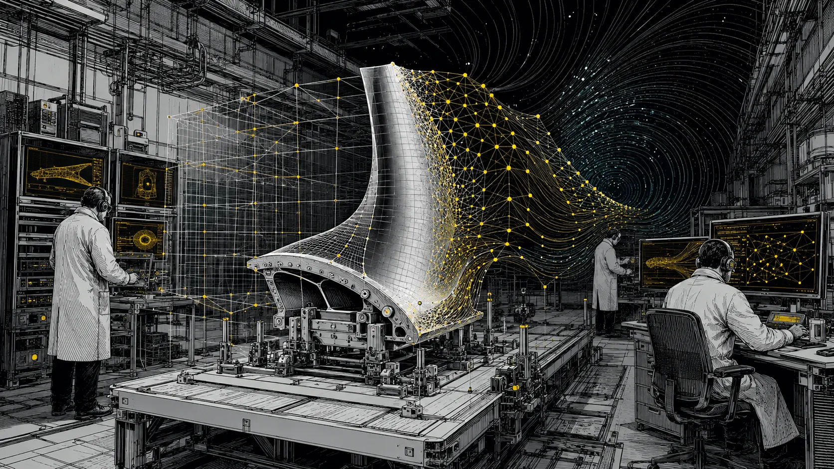
Yet the modern industrial landscape has encountered a hard computational wall. Engineering simulations traditionally require tens to hundreds of millions of spatial cells to discretise a given physical problem. Iterative solvers then grind through these massive geometric meshes, computing state changes across minute time steps. As demand for rapid prototyping, real-time digital twins, and instant design-space exploration escalates, the fundamental latency of mesh-based iterative solvers has become an insurmountable bottleneck.

A profound technological shift is underway — transitioning the industry from classical numerical analysis toward Physical Artificial Intelligence (Physical AI). Driven by advances in differentiable programming and the invention of Neural Operators, the simulation ecosystem is evolving from discrete grid-based approximations toward continuous, infinite-dimensional functional mappings.

The History of Numerical Analysis

The development of numerical analysis was not initiated by the electronic computer. It was born out of the fundamental human need to find approximate solutions to mathematical problems that defied exact analytical resolution. The earliest recorded numerical algorithms date back to the ancient Babylonians, who documented iterative methods for calculating complex planetary orbits on cuneiform tablets.

The discipline matured significantly during the mathematical renaissance of the 18th and 19th centuries through the work of Euler, Gauss, and Lagrange. By 1800, Lagrange polynomials were actively used for mathematical approximation; by 1900, Gaussian elimination was in common scientific use. During this era, a "computer" was a human mathematician performing gruelling manual calculations — a tradition famously depicted in the story of the Hidden Figures mathematicians of the early space programme.

World War II, the Space Race, and the Birth of Scientific Computing

The true inflection point arrived during the mid-20th century. The need to calculate artillery trajectories, nuclear reactions, and aerodynamic loads drove the transition from human hand-calculation to automated digital systems. The National Bureau of Standards, heavily supported by the Office of Naval Research, established the Institute for Numerical Analysis (INA) at UCLA in 1948, tasking it with developing algorithms specifically optimized for electronic computers.

This period spawned early software precursors to modern environments like MATLAB and Maple, pioneered by figures like Cleve Moler, who sought to make advanced matrix computations accessible to the broader engineering community. Domain-specific tools like SPICE for electrical circuit analysis revolutionised their respective fields.

The Industrial Forging of the Finite Element Method

The Finite Element Method (FEM) — which became the cornerstone of modern structural and continuum-media analysis — emerged through simultaneous, independent theoretical breakthroughs in applied mathematics and aerospace engineering.

The mathematical foundation was laid in 1943 by Richard Courant, who utilised the Rayleigh-Ritz method with trial functions defined on finite triangular subdomains to solve second-order PDEs. Independently, in 1941, Alexander Hrennikoff modelled continuous membranes as discrete lattice frameworks of bars and beams — a primitive but effective early form of the method.

However, the modern scalable engineering application of FEM was forged in the aerospace industry. In the early 1950s, engineers at Boeing, led by M. J. Turner, discretised delta-wing aircraft structures into interconnected mathematical "elements" to determine complex stresses and deflections that analytical models of the time could not handle.

Ray W. Clough of UC Berkeley, working at Boeing in 1952, recognised the profound implications of this approach. His landmark 1960 paper officially coined the term "Finite Element Method" — a phrase that instantly resonated due to its descriptive clarity. Across the Atlantic, John H. Argyris at Imperial College London translated Courant's variational mathematics into practical energy methods for engineering structures.

This foundational work ultimately spawned the multibillion-dollar commercial engineering software industry: NASTRAN, ANSYS, ABAQUS, COMSOL, and others. These platforms expanded beyond structural mechanics to encompass finite volumes, boundary elements, and meshfree methods across a vast landscape of coupled multiphysics problems.

Differentiable Physics: The New Frontier

For over half a century, writing a highly efficient custom PDE solver was an arduous, highly specialised task — demanding deep expertise in numerical discretisation schemes, advanced linear algebra, and low-level C or Fortran programming. Today, this dynamic has been completely inverted.

What Is Automatic Differentiation?

Automatic differentiation (autodiff) must not be confused with numerical differentiation (which approximates derivatives via finite differences and suffers from truncation errors) nor symbolic differentiation (which attempts exact algebraic expressions but suffers from exponential expression swell). Instead, autodiff applies the fundamental chain rule of calculus directly to the elementary algorithmic operations executed in a computer program, computing exact gradients through massive, complex software pipelines.

Frameworks like Google JAX have revolutionised scientific computing by combining NumPy-like Python syntax with Just-In-Time (JIT) compilation via the XLA compiler and native autodiff support across GPUs and TPUs. If a simulation developer writes a Python function f that evaluates a mathematical expression, passing it through jax.grad(f) automatically generates an exact gradient function. Developers can apply this transformation iteratively to compute higher-order derivatives with minimal code overhead.

Method	Accuracy	Speed	Scalability
Numerical Diff.	Low (truncation)	Slow	Poor
Symbolic Diff.	Exact	Very slow	Expression swell
AutoDiff (AD)	Exact	Fast	Excellent ✓

The Differentiable Physics Ecosystem

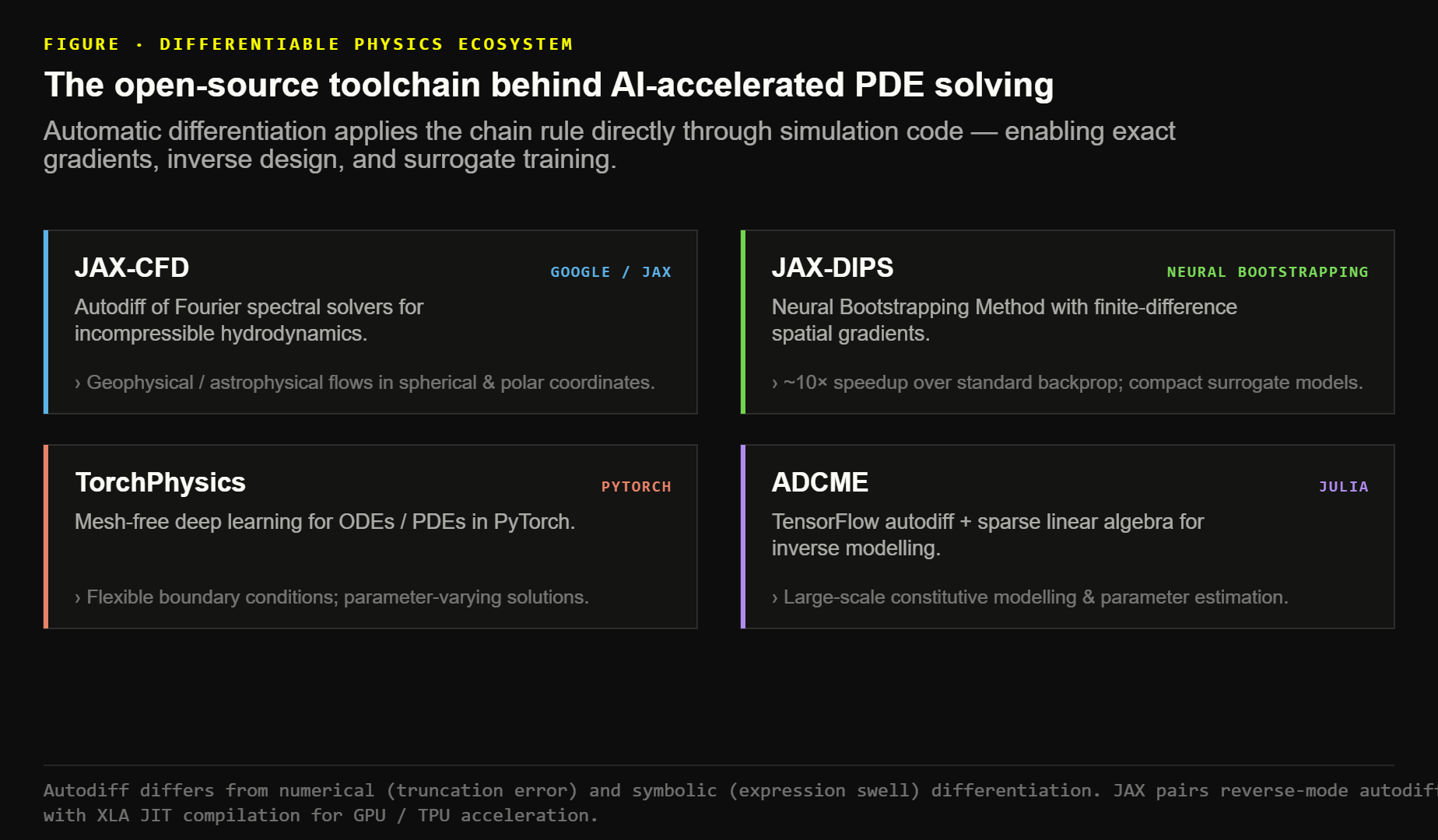
This capability has birthed a new ecosystem of differentiable PDE solvers that bridge classical numerical analysis and modern machine learning:

Framework	Key Innovation	Benefit
JAX-CFD	Autodiff of Fourier spectral solvers for incompressible hydrodynamics	Geophysical / astrophysical flows in spherical/polar coordinates
JAX-DIPS	Neural Bootstrapping Method (NBM) with finite-difference spatial gradients	10× speedup over standard backpropagation; compact surrogate models
TorchPhysics	Mesh-free deep learning for ODEs/PDEs in PyTorch	Flexible boundary conditions; parameter-varying solutions
ADCME (Julia)	TensorFlow autodiff + sparse linear algebra for inverse modelling	Large-scale constitutive modelling and parameter estimation

Table 1 — Key differentiable physics frameworks and their innovations.

Inverse Design — By allowing mathematical gradients to flow backward through time-steps of a numerical simulation, differentiable solvers enable "inverse design": instead of running thousands of forward simulations in a trial-and-error loop, engineers define a desired output state and the autodiff system calculates the exact initial parameters or geometries required to achieve it. This transforms optimisation from a heuristic guessing game into a deterministic mathematical calculation.

The Architectural Revolution: Neural Operators

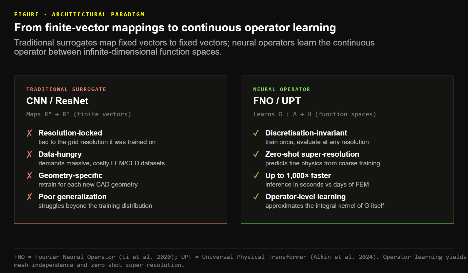
While differentiable programming optimises classical numerical algorithms, the most profound breakthrough in contemporary Physical AI is the circumvention of grid-based iterative solving entirely. Traditional machine learning initially attempted to address simulation latency via Surrogate Modelling — training standard CNNs or ResNets on large FEM/CFD datasets to approximate outputs.

While offering lower compute at inference time, traditional surrogates suffer from severe mathematical limitations: they map finite-dimensional vectors to other finite-dimensional vectors, remaining tightly coupled to the specific grid resolution they were trained on. They struggle to generalise beyond training distributions, demanding massive datasets that are prohibitively expensive to generate.

The Mathematical Framework

Neural Operators fundamentally shift this paradigm. Instead of mapping between discrete finite vectors, Neural Operators learn continuous mappings between infinite-dimensional function spaces. If a classical PDE is defined by a physical operator 𝒢 mapping an input function a ∈ A to a solution function u ∈ U, the Neural Operator approximates the integral kernel of the operator 𝒢 itself.

Because they learn the continuous operator underlying the physics, these models achieve discretisation-invariance (mesh-independence). Once fully trained, a Neural Operator can be evaluated at any arbitrary spatial or temporal resolution without retraining — effectively decoupling physics prediction from the geometric grid entirely.

The Fourier Neural Operator (FNO)

The watershed moment arrived when Li et al. (2020) introduced the Fourier Neural Operator (FNO). The FNO parameterises the integral kernel of a PDE directly in Fourier space. By computing continuous convolutions via the Fast Fourier Transform (FFT), FNOs successfully learn mappings from any parameterised PDE input to its rigorous physical solution.

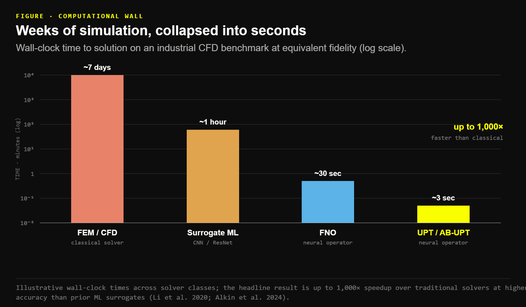
The empirical results are staggering: FNOs perform zero-shot super-resolution on highly complex turbulent flows, achieving up to 1,000× computational speedups over traditional solvers while maintaining significantly higher accuracy than any prior ML-based surrogate methods. A model trained on coarse-resolution data correctly predicts fine-resolution physics without ever having seen it — a property impossible for classical surrogates.

The Universal Physical Transformer (AB-UPT)

Taking Neural Operators further into industrial scalability, Alkin et al. (2024) developed the Universal Physical Transformer (UPT). The architecture follows a generic "encode–propagate–decode" paradigm:

• Encoder: Complex input geometries (CAD files, point clouds) are compressed hierarchically. Points are clustered into "supernodes" via graph pooling, then flattened to a fixed token count via Perceiver-style attention.
• Approximator: A deep Transformer stack propagates latent tokens across discrete space and time. For transient problems, tokens are updated in a recurrent or autoregressive fashion.
• Decoder (Neural Field): A cross-attention neural field maps latent tokens back to the physical domain. Crucially, the decoder is evaluated point-wise — querying at arbitrary spatial coordinates does not increase the computational complexity of latent propagation.

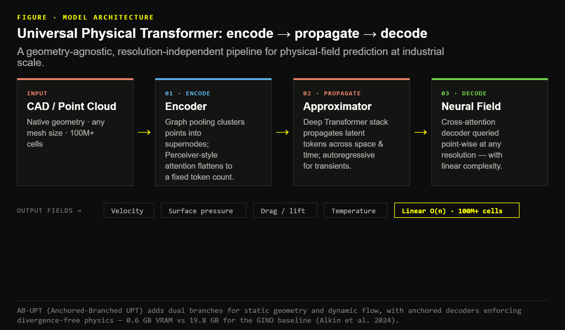
The refinement into AB-UPT (Anchored-Branched UPT) introduced a multi-branch architecture with separate branches for static geometry features and dynamic flow features, synthesised later in the pipeline. Anchored neural field decoders enforce divergence-free flow physics and scale inference to industrial meshes containing over 100 million cells with strictly linear computational complexity.

AB-UPT performance benchmarks on industrial ShapeNet and DrivAer datasets: 1,000× speedup vs classical solvers · under 24 hrs training on a single GPU · 100M+ cells at linear complexity · 0.6 GB VRAM vs 19.8 GB for the GINO baseline.

Real-World Industrial Applications

Automotive and Aerospace Aerodynamics

Airflow simulation for vehicle and aerodynamic design is the primary commercial target for Neural Operators. Catalani et al. (2026) demonstrated that neural field surrogates can predict 2D airfoil flows with an order-of-magnitude higher accuracy than prior models, successfully handling full aircraft wing meshes. AB-UPT specifically targeted passenger car aerodynamics via the DrivAer datasets, predicting surface pressure, volumetric velocity fields, and drag/lift coefficients at strict industrial fidelity. Engineering teams can now perform interactive design exploration — evaluating thousands of geometric configurations in minutes, fundamentally altering the aerodynamics development lifecycle.

Additive Manufacturing and Digital Twins

The realisation of real-time digital twins for complex manufacturing processes is now viable. Liu et al. (2024) constructed an FNO-based surrogate for Laser Powder Bed Fusion (L-PBF) additive manufacturing. Their model learns the complete melt-pool temperature field as a direct function of laser power. Because inference occurs in milliseconds, the system enables closed-loop control: it can predict defect-inducing thermal conditions on the fly and adjust laser parameters dynamically to prevent part failure, all while providing probabilistic uncertainty estimates.

Granular and Particulate Flows

Many critical industries — pharmaceuticals, food processing, industrial chemicals — rely heavily on fluidised beds and particulate hoppers. Traditional coupled DEM-CFD simulators are notoriously slow. NeuralDEM, the first end-to-end deep surrogate for coupled particulate flows, models complex hopper outflows and fluidised-bed mixing in real time across multiple flow regimes, handling millions of particles and hundreds of thousands of fluid cells simultaneously. The model and dataset were made open-source in September 2025, democratising reactor digital twins.

Structural Dynamics, Materials, and Energy Grids

Neural Operators extend well beyond fluid dynamics. Zhou et al. (2024) applied operator networks to structural vibration analysis, training a surrogate that accurately predicts time-varying structural responses from material properties and external excitation parameters — facilitating rapid system identification and inverse parameter derivation. At the macro scale, FNOs and DeepONets have been applied to super-parameterise global climate models and stabilise complex power grid PDEs, demonstrating the relevance of operator mathematics from microscopic metamaterials to planetary and electrical systems.

Conclusion: The End of the Mesh Era

We are witnessing the end of the mesh era. Neural Operators do not merely accelerate existing simulation workflows — they fundamentally reimagine what physical prediction means. The ability to learn continuous physics operators, evaluate them at arbitrary resolutions, and do so in seconds rather than days is not an incremental improvement. It is a categorical change in the relationship between computation and physical reality.

The convergence of differentiable programming, Fourier Neural Operators, and Transformer-based Physical AI architectures represents the most significant shift in engineering simulation since FEM was coined in 1960. The historical journey — from Babylonian cuneiform tablets to Gaussian elimination, from Boeing's delta-wing problem to NASTRAN, from ANSYS to JAX-CFD, and now to FNOs and AB-UPT — traces a consistent arc: the relentless democratisation of physical prediction.

Neural Operators are no longer academic curiosities. They are actively penetrating industrial sectors, compressing simulation timelines from weeks to seconds, enabling true real-time digital twins, and unlocking closed-loop process control at industrial scale. The engineering teams, software platforms, and organisations that embrace this transition earliest will hold a decisive competitive advantage.

The mesh era is ending. The era of Physical AI has begun.

---

Keywords: Physical AI, Neural Operators, Fourier Neural Operator, FNO, Finite Element Method, FEM, CFD, Differentiable Physics, UPT, AB-UPT, Digital Twins, Deep Learning, Engineering Simulation, JAX, Autodiff

© 2025 DeepMechanix · References available on request.